VLOOKUP is a great tool for pulling data from tables, but it has a handicap: it can only work with one criteria for matching information. If there are multiple rows in your sheet with the same information, you’ll only get the first one. If you need to use two or more conditions to match a specific piece of data, you’re out of luck. Fortunately, Excel has a pair of functions called INDEXand MATCH that can help produce the same results as VLOOKUP with multiple criteria. Here’s a quick tutorial to help you learn how…
Quick Navigation [hide]
Example Data
Let’s say, for example, that we want to be able to search through a list of fuel economy data for cars to find the mileage…
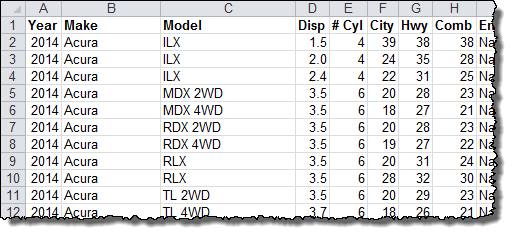
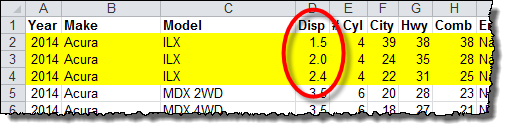
Normally, we would want to be able to enter the model of a car and get it’s fuel economy as a result. Unfortunately, Many cars, like the Acura ILX, have multiple engine configurations with different mileage ratings. Fortunately, in this case, the car’s displacement can serve to separate them.
This means, however, that we will need to look up the car by both its Model and its Displacement at the same time to find the appropriate Combined Fuel Economy in column H.
Trying to Use VLOOKUP
In a normal VLOOKUP, the syntax is as follows:
=VLOOKUP(lookup_value, table_array, col_index_num, [range_lookup])
The lookup_value is the data you are searching with.
The table_array defines the table that you want to look through. The first column must be the column that has the lookup_value in it.
The col_index_num is the number of the column in the table_array that has the data you want to find.
The optional range_lookup specifies whether the list is sorted or not. (TRUE means that VLOOKUP stops looking when it finds something that comes later in the alphabet than the lookup_value. FALSE means it searches the entire list.)
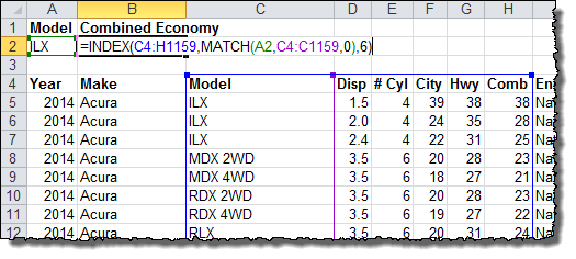
If we were looking for just the Model of car using VLOOKUP in our example data, it would look like this:
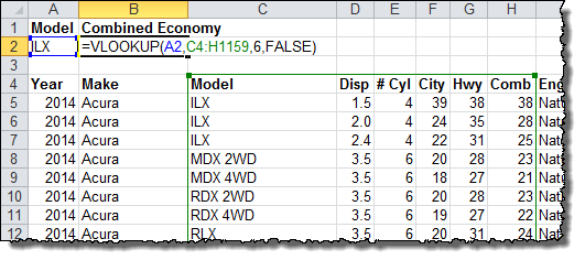
=VLOOKUP(A2,C4:H1159,6,FALSE)
A2 holds the Model of car we want to find.
C4:H1159 is the table we want to search through. Column C is the column with the Model information.
Column 6 is the column that holds the Combined Fuel Economy figure that we want to find.
The result of the VLOOKUP is this:
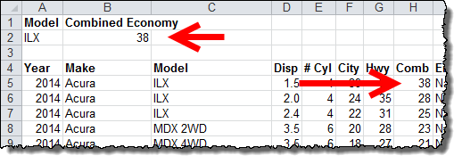
It finds the first entry that matches – the 1.5 liter engine with 38 MPG. This is a problem if, for example, you want to find the fuel economy of the 2.4 liter sport version. To do that, we need to use INDEX and MATCH.
Using INDEX and MATCH to Replace VLOOKUP
What we really need is to be able to look up the Model and the Displacement at the same time. MATCH is a function that gives you the location of an item in an array. The syntax for MATCH is as follows:
=MATCH(lookup_value, lookup_array, [match_type])
The lookup_value is what you are searching for.
The lookup_array is the array of values you are trying to find the lookup_value in.
The optional match_type determines whether MATCH must find the lookup_value exactly (with a 0), or return the closest match that comes before it (with a 1) or after it (with a -1) alphanumerically.
The INDEX function takes a location and returns the value that is in the cell. The syntax for INDEX is as follows:
=INDEX(array, row_num, [col_num])
The array is the table of data that contains the cell value you want.
The row_num is the relative row number of the cell you want.
The col_num is the relative column number of the cell you want.
By combining INDEX and MATCH we can produce the same result as VLOOKUP. Using the same search we did forVLOOKUP, the INDEX/MATCH pair looks like this:
=INDEX(C4:H1159,MATCH(A2,C4:C1159,0),6)
C4:H1159 is the array that INDEX uses to find the value.
A2 is the cell that the value we want MATCH to find.
C4:C1159 is the lookup_array that MATCH looks through to find the value in A2.
The 0 means that MATCH will look for the exact value instead of an approximate one.
Column 6 is the column in the C4:H1159 array that holds the Combined Fuel Economy values.
The result is identical to the VLOOKUP result. MATCH finds the first Combined Fuel Economy value for the Acura ILX, which means it will give 38 MPG for the 1.5 instead of one of the other engine options. To find a specific Modeland engine Displacement combination, we need to modify our INDEX/MATCH formula into an array formula.
Using INDEX and MATCH with Two Criteria
To allow MATCH to search for multiple criteria, we are going to change the way it looks for its result by making it an array formula.An array formula takes an array of values instead of a single one and checks each cell in the array until it finds a result.
Our old MATCH formula looked like this:
=MATCH(A2,C4:C1159,0)
It looked for the value of A2 in the table C4:C1159, and when it found it, it returned the location.
Now we are going to ask it to be creative:
=MATCH(1,(C4:C1159=A2)*(D4:D1159=B2),0)
We have asked MATCH to look for a value of 1. Instead of giving it an existing array to look through, we are asking it to build one from scratch. The new array checks all the values in C4:C1159 for one that matches A2 and all the values in D4:D1159 for one that matches B2. Where they both match, the array will have a 1 (a TRUE boolean result). Where they don’t both match, the array will have a 0 (a FALSE boolean result). Therefore, MATCH will return the location where the array matches 1 (when both of our criteria are true).
If this process doesn’t make sense to you, that’s okay. Just plug the new MATCH function into your INDEX/MATCHformula:
=INDEX(C4:H1159,MATCH(1,(C4:C1159=A2)*(D4:D1159=B2),0),6)
When you enter the formula, don’t just press ENTER. Press CTRL+SHIFT+ENTER to tell Excel that it is an array formula. You can tell you’ve done it right because the entered formula will be surrounded in curly braces {}.
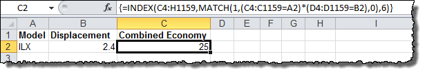
With that, your formula will be able to find the Combined Fuel Economy based on both the Model and the Displacement. You can use this technique for any number of criteria with INDEX and MATCH. Just add additional terms to the multiplication equation.
Multiple Criteria VLOOKUP with INDEX and MATCH Example Download
You can follow along with this tutorial using the original source data and explore an example of the solution in the embedded file below. To download your own copy, click on the green Excel icon in the lower right corner.
No comments:
Post a Comment